

The frequency-following response (FFR) is a neurophysiological response to sound that precisely mirrors the temporal dynamics of the auditory stimulus. The frequency-following response (FFR) is believed to originate in the brainstem and is typically recorded from the scalp at the Cz electrode site, which corresponds to the cortical projection of the inferior colliculus [2]. The FFR serves as a valuable tool for investigating the integrity and plasticity of neural sound encoding across the lifespan. Pathologies may disrupt central auditory processing, whereas acquired experience can enhance it. The FFR enables the assessment of the neural consequences of language deprivation, autism, concussion, and reading impairments. It captures the effects of enriched auditory experiences, including short-term training, bilingualism, and musical practice [3].
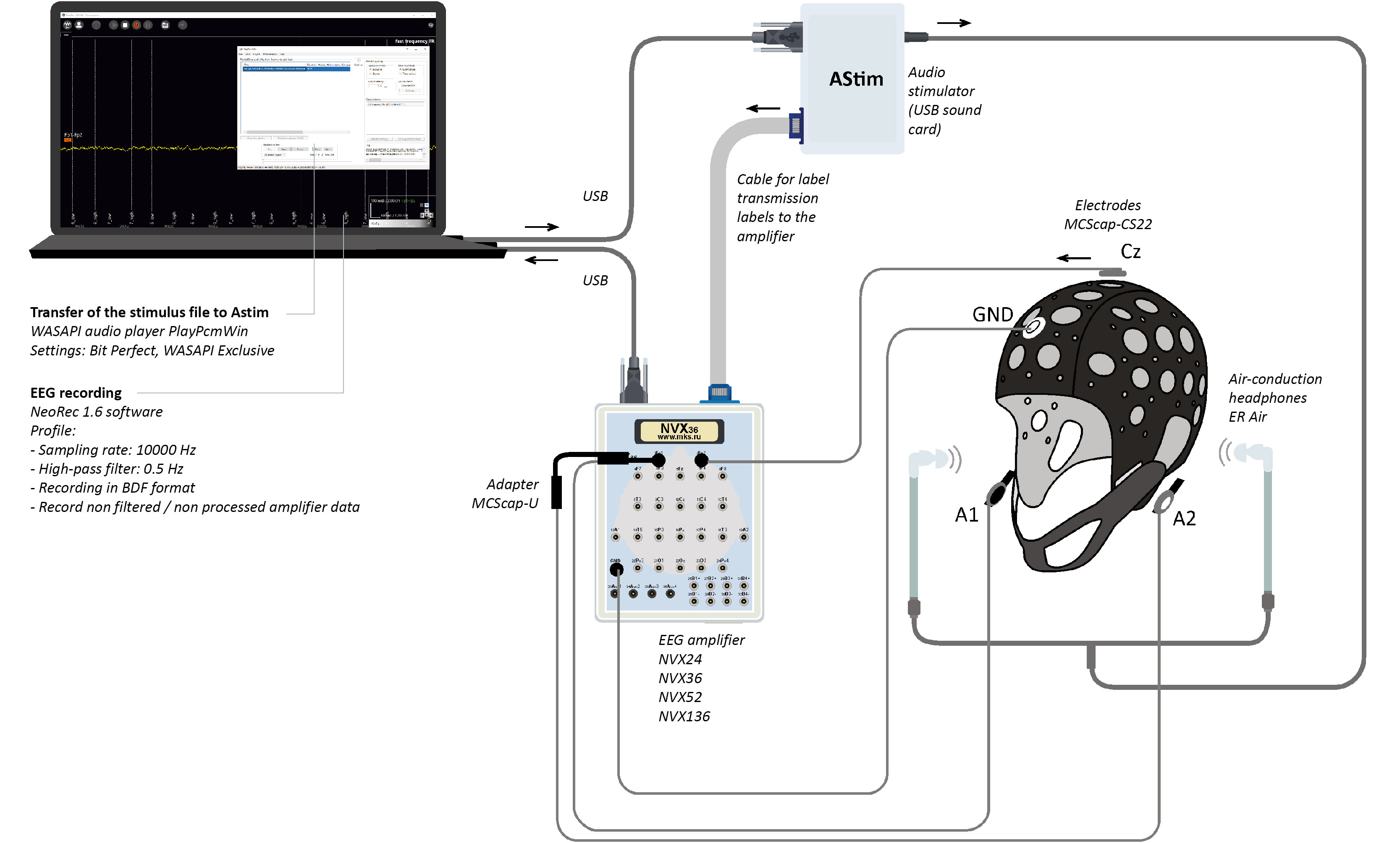
A prototype FFR monitor was developed using MCS hardware and software. This system generated and delivered an acoustic stimulus with predefined characteristics to the participant, from which the frequency-following response (FFR) was recorded as an evoked potential.
- At a sampling rate of 10000 Hz, the temporal jitter remained below 1 ms. The rate of event trigger losses was less than 0.0002 % of the total number of triggers.
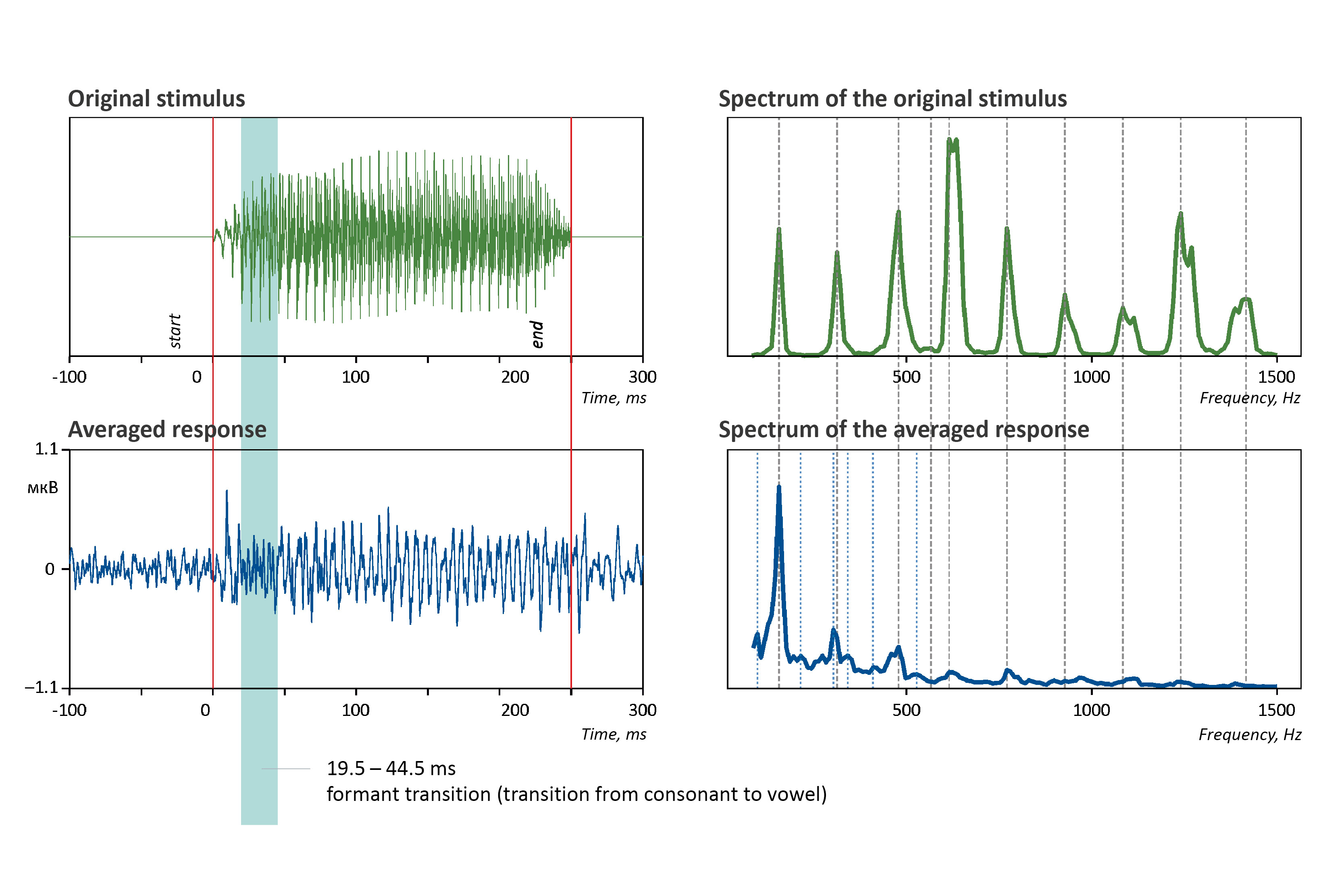
- The amplitude of the recorded evoked potential fell within the anticipated range of ±0.2 µV [3]. Spectral analysis revealed that up to 50 % of the amplitude peaks in the evoked response matched the spectral characteristics of the presented auditory stimulus.
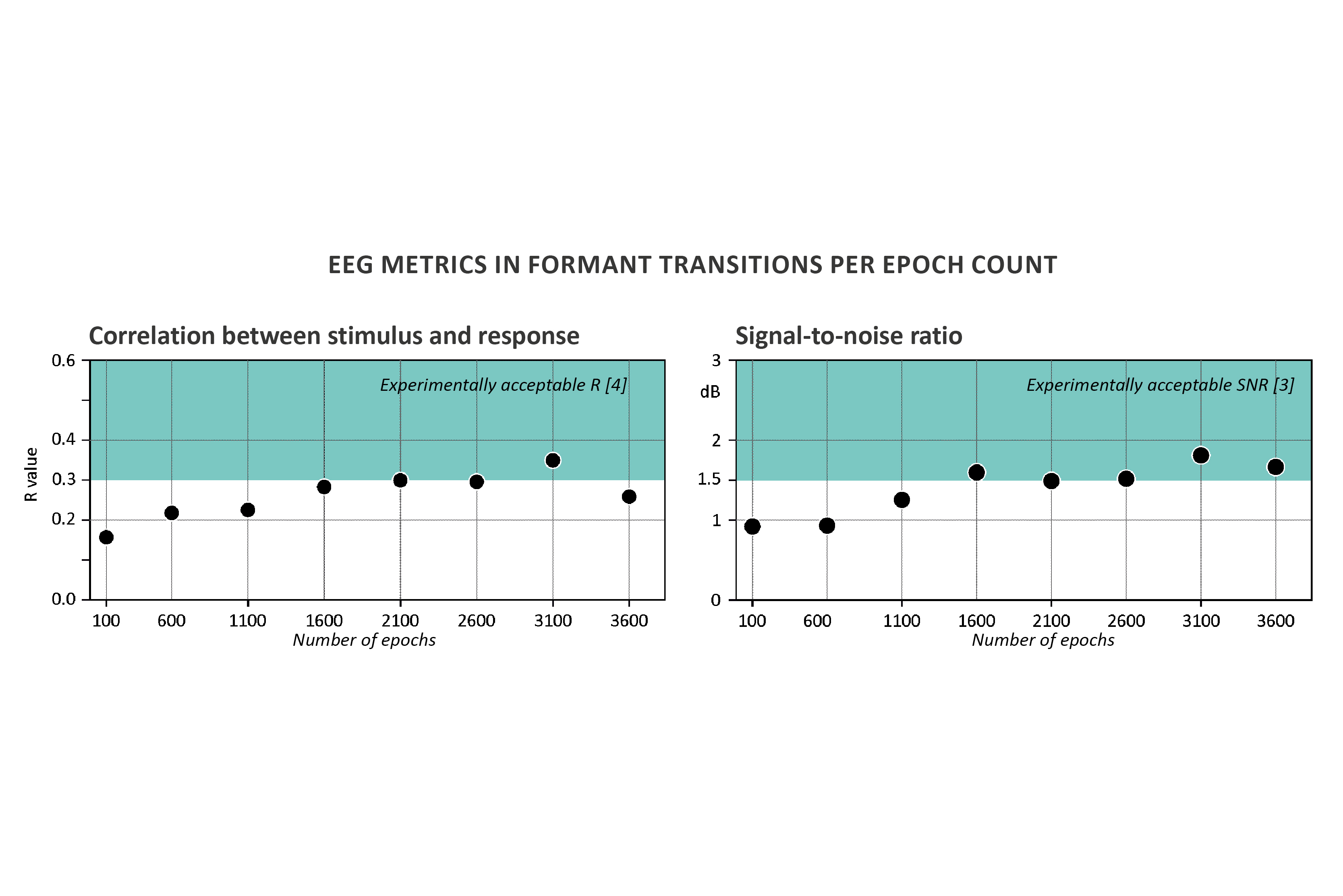
- To assess stimulus–response correspondence, we calculated the Pearson correlation coefficient between the stimulus waveform and the evoked FFR within the formant transition window (19.5–44.2 ms relative to FFR onset). This analysis accounted for the physiological lag of 7–9 ms due to signal propagation from the ear to midbrain structures. As the number of averaged epochs increased, the correlation rose accordingly and attained previously reported levels (r > 0.3) [4].
Equipment
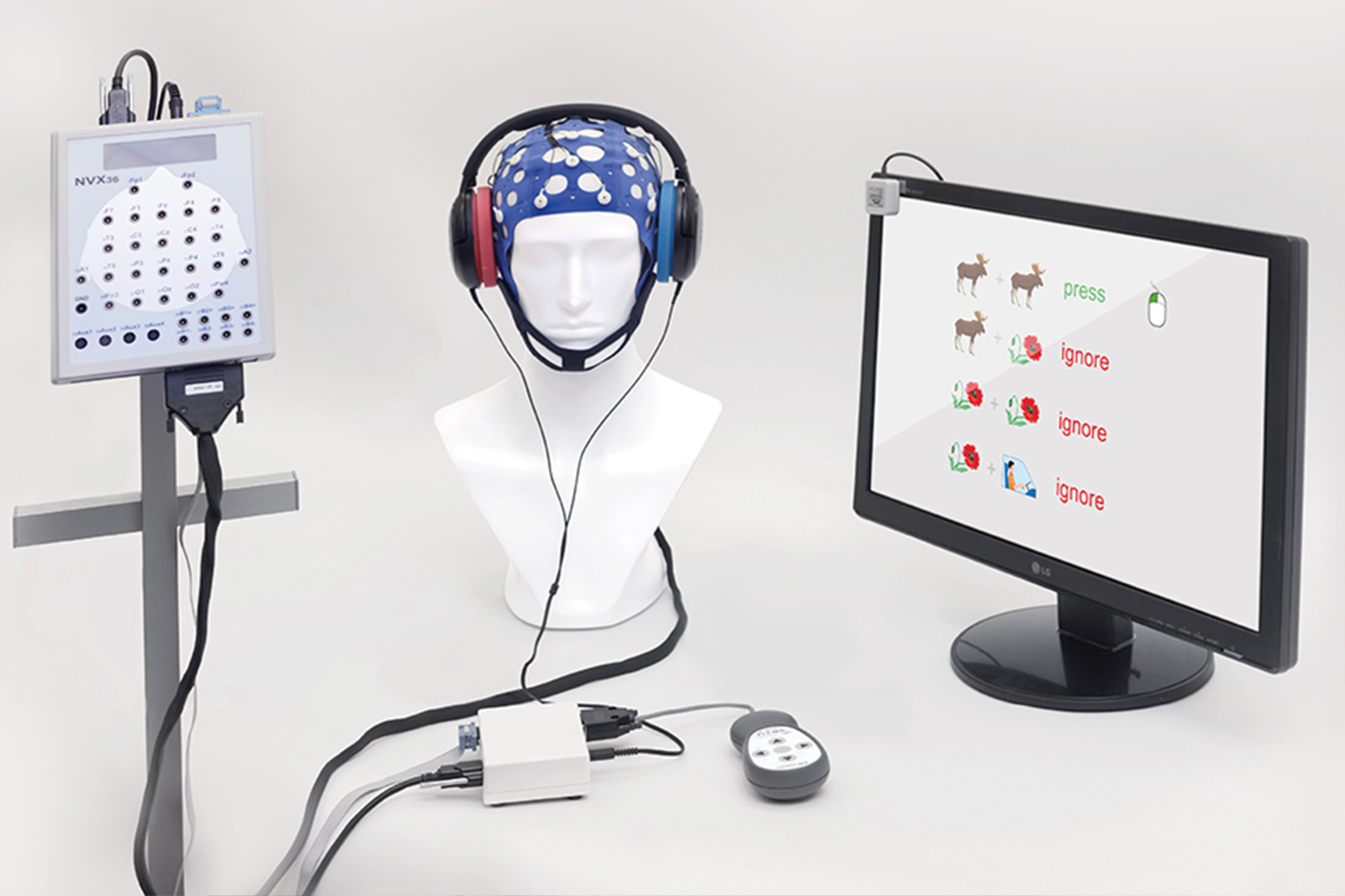
- a single-channel EEG recording was performed using the MCScap system with MCScap CS22 electrodes: active electrode at Cz, ground (GND), and reference at the averaged mastoids (Ref (A1 + A2)/2);
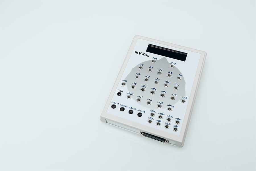
- EEG amplifier NVX36 or NVX136 (high-resolution channels were used: Cz->Fp1, Ref->Fp2, GND->GND);
- preamplifier MNSENS-ACP;
- acoustic stimulator ASTIM;
- anti-radiation 3.5mm Air Acoustic Tube Earpiece Headset acoustic headphones;
- geltek Unimax.
Software
- NeoRec 1.6;
- project FFR (Frequency_Following_Response_Astim Version 1);
- playPcmWin player (64-bit).
EQUIPMENT & SOFTWARE
EXPERIMENT DESCRIPTION
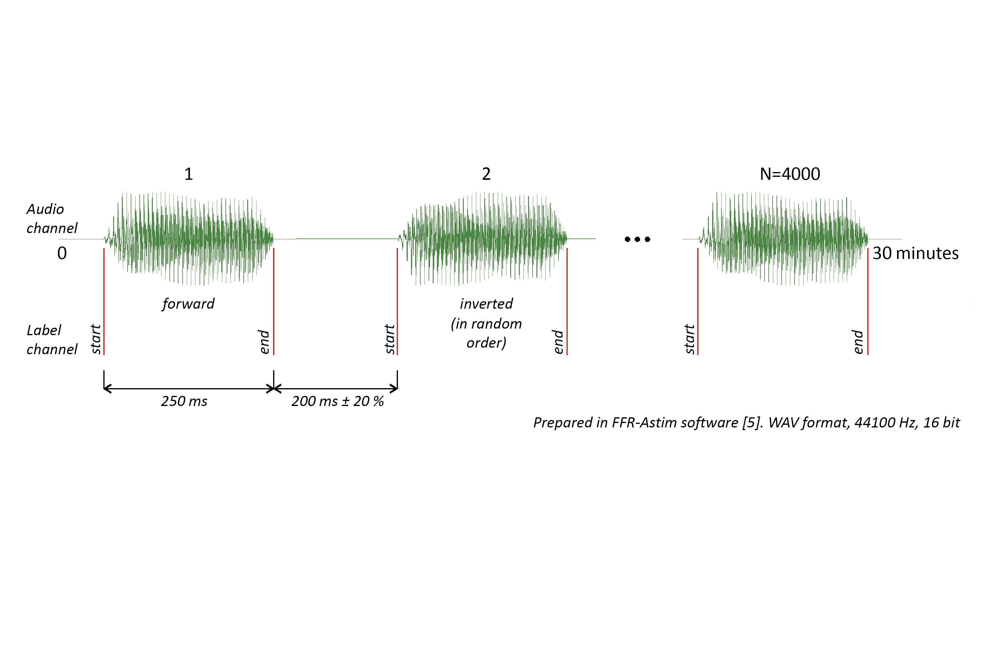
The audio file was created by the Project FFR software in .wav format with a dedicated channel for marker transmission. To eliminate bone artifacts, two types of stimuli were used — original (6 low) and amplitude-inverted (7 low) [3]. The audio file consists of 4000 repetitions of the syllable "Da" (2000 repetitions of the original stimulus, 2000 repetitions of the inverted one), separated by pauses. The stimulus duration is 250 ms, and the inter-stimulus interval duration is 200 ms ±10 %. The stimulus was delivered to the ASTIM in bit-perfect WASAPI Exclusive mode with full sound card capture using the PlayPcmWin player (64-bit).
The player's buffering (output latency) was 170 ms. The sound transmission delay through the headphone tubes was 0.7 ms. In the preliminary stages of the experiment, the sound pressure level SPL during stimulus playback was 78 dB.
The subject was comfortably seated in a chair in a semi-dark room, relaxed, with eyes open. Reading from a phone or laptop was permitted [4]. The experiment duration was 32 minutes.
One electrode was placed at location Cz, one - Gnd, and the reference (A1 + A2)/2 (on the earlobes). The impedance value on the Cz channel was 13 kΩ.
EEG was recorded at a sampling rate of 10 000 Hz. During EEG recording, a MNSENS-ACP preamplifier with a gain of 500 and filtering of 16–3000 Hz, and an NVX36 amplifier were used.
During the experiment, a high-pass filter was applied to suppress the signal below 0.5 Hz. The data were saved in .bdf format and in raw data format.
DATA PROCESSING
Special software, Project FFR (Frequency_Following_Response_Astim), was developed in the Python language for stimulus preparation, signal processing, and data analysis [5].
Preparation of the .WAV file for stimulation
- import of the reference stimulus;
- creation of an amplitude-inverted stimulus;
- creation of markers for the start and end of the stimulus in the second audio channel, indicating whether the stimulus is direct or inverted;
- creation of a recording with an equal number of direct and inverted tokens arranged in random order, separated by pauses of random length 200 ms ±10 %.
Raw data cleaning
- verification of marker matching between the stimulus WAV file and the EEG;
- filtering 80 – 1500 Hz, 2nd-order Butterworth [3], [2];
- segmentation from –100 ms before stimulus onset to 300 ms after stimulus onset;
- removal of artifact epochs with signal amplitudes >40 µV [1];
- averaging across all artifact-free epochs relative to stimulus onset.
Analysis
Spectral amplitude is calculated using the Fourier transform (Welch's method) [4] with parameters: n_fft = 1024, n_per_seg = 1024, n_overlap = 512 (50 % overlap). At a sampling rate of fs = 10000 Hz, this provides a frequency resolution of Δf≈9.77 Hz.
Peak spectral amplitudes and frequencies for visualization were determined based on 10–12 peaks of the stimulus file/data, spaced no closer than 30 Hz from each other. From these peaks, the frequencies of the stimulus and FFR are selected with a corridor of ± 10 Hz (up to 20 Hz distance from stimulus peak to response peak).
The Pearson correlation coefficient between the stimulus and the response in the formant transition interval [3] was determined at different numbers of averages (starting from 100 and then in steps of 500). The calculation took into account a lag of 7–10 ms relative to the stimulus, as the signal transit time along the auditory pathways [1].
The signal-to-noise ratio SNR in the formant transition interval was also determined at different numbers of averages. RMS_signal was calculated over the interval_signal 19.5–44.2 ms [3] using the formula RMS_signal = (sum(interval_signal ** 2) / len(interval_signal)) ** 0.5. RMS_noise was calculated over the interval from –30 ms to 0 relative to stimulus onset: RMS_noise = (sum(interval_noise ** 2) / len(interval_noise)) ** 0.5. SNR was calculated as SNR = RMS_signal / RMS_noise.
EQUIPMENT
RESOURCES
[1] Coffey EBJ, Arseneau-Bruneau I, Zhang X, Baillet S, Zatorre RJ. Oscillatory Entrainment of the Frequency-following Response in Auditory Cortical and Subcortical Structures. J Neurosci. 2021 May 5;41(18):4073-4087. doi: 10.1523/JNEUROSCI.2313-20.2021.
[2] Gnanateja GN, Rupp K, Llanos F, Remick M, Pernia M, Sadagopan S, Teichert T, Abel TJ, Chandrasekaran B. Frequency-Following Responses to Speech Sounds Are Highly Conserved across Species and Contain Cortical Contributions. eNeuro. 2021 Dec 23;8(6):ENEURO.0451-21.2021. doi: 10.1523/ENEURO.0451-21.202.
[3] Krizman J, Kraus N. Analyzing the FFR: A tutorial for decoding the richness of auditory function. Hear Res. 2019 Oct;382:107779. doi: 10.1016/j.heares.2019.107779.
[4] Skoe E, Kraus N. Auditory brain stem response to complex sounds: a tutorial. Ear Hear. 2010 Jun;31(3):302-24. doi: 10.1097/AUD.0b013e3181cdb272.
[5] ПО Frequency_Following_Response_Astim Version 1. Репозиторий проекта: https://github.com/asmyasikova83/Frequency_Following_Response_Astim.